Reflection photoelasticity

1. Building a reflective polariscope

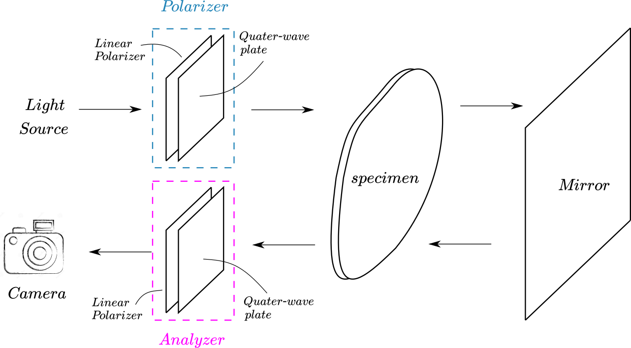
Reflective polariscopes allow for the visualization of the photoelastic fringes when the light source and the camera are located on the same side of the photoelastic specimen. As shown in the figure below, they consist of 5 basic elements: * A light source * A single polarizer, which is ideally a circular polarizer located between the light source and photoelastic specimen. This is shown with both of its parts: a linear polarizer plus a quarter-wave plate. * A reflective surface, that can be either a mirror below the sample or a coating on the particles. * An analyzer, which is a circular polarizer located between the photoelastic specimen and the camera. * A camera.

Similar to the transmissive polariscope, both the polarizer and the analyzer should be circular polarizers. In assembling the circular polarizers, it is important for the principle axis of the quarter-wave plate to make a $45^{\circ}$ angle with the direction of polarization of the linear polarizer. Note that for a darkfield polariscope, the analyzer must match the chirality of the polarizer on the incident light path (see section 2. for mathematical proof), and can even be the same optical element. For a brightfield polariscope, the two polarizers are complementary.

1.1. Example experimental realizations

There are two typical ways to implement the mirror in real granular physics experiments:

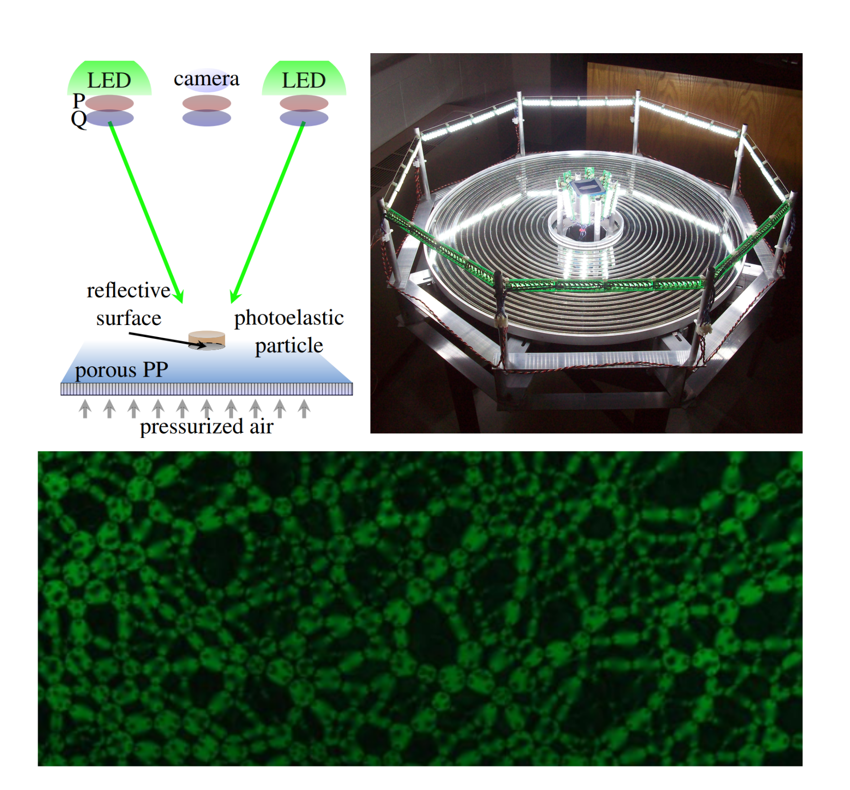
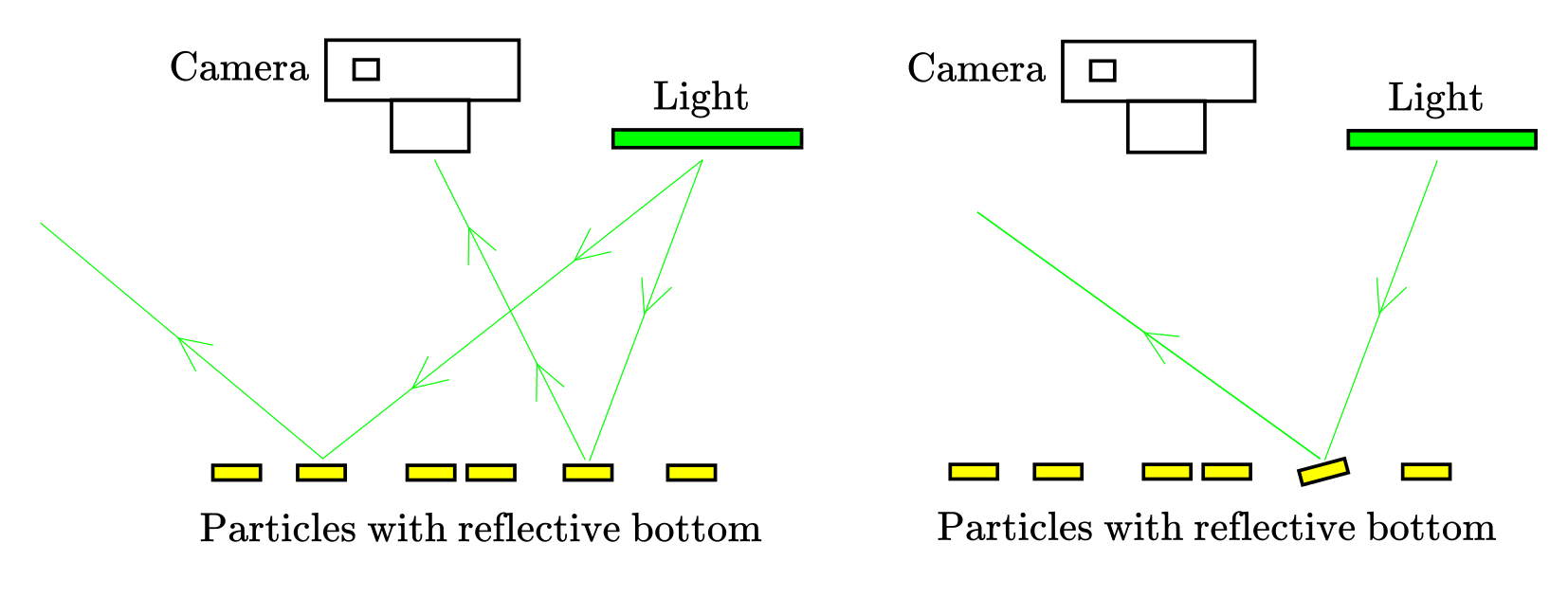
• Using photoelastic particles with one reflective surface. The left figure below shows a sketch of an example experimental setup using this technique. (see J. Puckett et al. or K. E. Daniels et al. for more details about the experiment) A typical image recorded from this experiment for a jammed disc packing is also attached below (from the Ph.D. Thesis of J. G. Puckett ), showing the same type of fringes as observed in the transmissive polariscopes.
• Using a mirror table. Transparent particles are then put on this table to perform experiments. This technique allows the usage of transparent photoelastic particles in the same way as in the transmissive polariscope case. An example implementation of the mirror table is shown in the up-right subfigure of the figure below. (see Y. Zhao et al. for more details of this experiment)

1.2. How to make the photoelastic particles reflective?

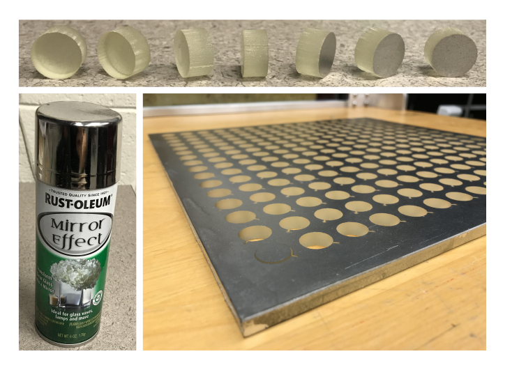
A typical way to create a reflective surface for photoelastic particles is to coat one side of the particles with mirror-effect paint. An empirical choice that works well is the Rust-Oleum Mirror Effect spray (figure below). To ensure uniform coating, it is typical to first paint a sheet of photoelastic material and then cut particles from it. The lower right figure below shows a picture of the painted photoelastic sheet after cutting of the particles. The figure below also shows different angles of particles after this coating process.

1.3. Determine the configuration of circular polarizers

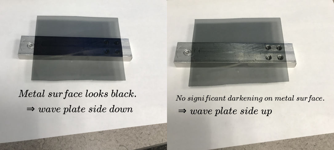
It is very important to note that in reflective polariscope, the circular polarizers used as both Polarizer and Analyzer must have their quarter-wave plate side towards the granular sample. However, sometimes it is hard to tell which side of a circular polarizer is a quarter-wave plate. A simple trick can be used to solve this problem: put the circular polarizer on a piece of metal (can be any metal in the lab, even your lab keys). If the metal becomes black then the wave-plate side is towards the metal, otherwise the linear polarizer side is towards the metal. (see section 2. for why)

1.4. Ensure a uniform distribution of light intensity

In experiments using photoelastic particles, it is important to keep the light intensity distribution uniform in the system. Because both empirical pressure measurement and the nonlinear fitting force measurement depend sensitively on the background light intensity. The reflective polariscope has a higher chance to suffer from light heterogeneity, compared to the transmissive polariscope. First, the reflection light intensity is more sensitive to the relative position between the light source, particle, and camera (left figure below). Second, if the effective mirror is implemented using coated particles, small tilting of particles may induce a big change in background light intensity for that particle (right figure below).

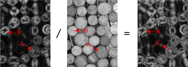
To reduce the light heterogeneity, the light source should have a large enough area. The light heterogeneity can also be reduced using the following trick. When taking photoelastic images using both Polarizer and Analyzer (left figure below), take another image without Analyzer while keeping everything else the same (middle figure below). The second image gives information about the background light intensity $I_0$ (see section 2 for details). Divide the first image using the second image results in a rescaled image with uniform light intensity (right figure below), which can be used in the data analysis afterward.

1.5. Coated particles or mirror table?

The painted surface of particles usually can not reflect light as well as a commercial mirror. However, the coated particles are irreplaceable in cases where a mirror table can not be used. For example, in air table experiments (see J. Puckett et al. for more details). The mirror table solution also has disadvantages. In particular, the mirror image of the particle boundaries will be recorded by a camera, creating additional difficulties for boundary detection. In most cases, coated particles work well enough. However, the mirror table solution remains a choice when coating particles is not practical (for example if the same particles are also used in other experiments with transmissive polariscope).

2. Theoretical background

In this section, the theoretical background of the reflective polariscope is reviewed. In section 2.1. the relation between local stress and the light intensity recorded by the camera is derived. In section 2.2. proof for the chirality change of circularly polarized light after reflection is presented.

2.1. Photoelasticity in the reflective polariscope

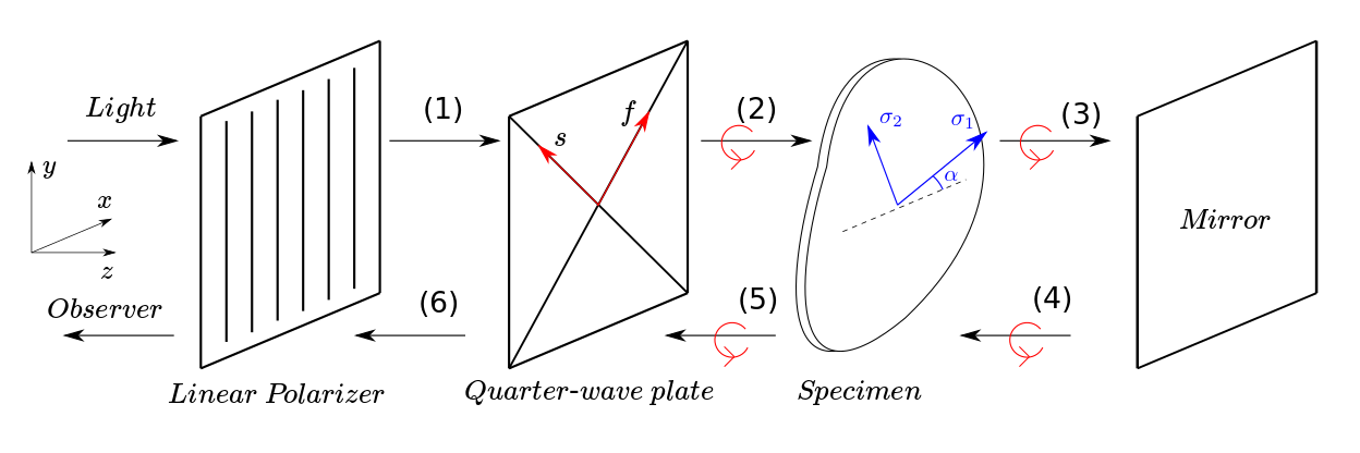
As shown in the above figure, under a reflective polariscope, the circularly polarized light goes through the photoelastic specimen twice with different chirality of polarization. Suppose the height (the size along $z$ direction) of the specimen is $h$, the pattern observed here will be the same as the pattern formed by a $h/2$ height specimen using transmissive polariscope. This can be shown as following: suppose the linear polarizer creates a polarized light along $\hat{y}$ direction. In region (1) denote the light vector as: $$E_1 = \sqrt{I_0}e^{i(kz-\omega t)}\hat{y}$$ where $I_0=|E_1|^2$ is a constant called the background light intensity, $k$ is the wave number and $\omega$ is the frequency of the light. Suppose the principle direction for the stress tensor of the specimen point under consideration is $\hat{m_1}$ and $\hat{m_2}$ (corresponding to principle stress $\sigma_1$ and $\sigma_2$ respectively). Denote $\phi = \alpha - \pi/4$. Then in region (2) $$E_{2} = \frac{1}{\sqrt{2}}\sqrt{I_0}e^{i(kz-\omega t)}(-i\hat{f}+\hat{s}) = \frac{1}{\sqrt{2}}\sqrt{I_0}e^{i(kz-\omega t)}e^{i\phi}(-i\hat{m_1}+\hat{m_2})$$ where $\hat{f}$ and $\hat{s}$ are the fast and slow principle directions of the quarter-wave plate. Passing the specimen results in a $\Delta = 2\pi(\sigma_1-\sigma_2)/f_{\sigma}$ phase lead [5] to the $\hat{m_1}$ component of light. So in region (3):
$$E_{3} = \frac{1}{\sqrt{2}}\sqrt{I_0}e^{i(kz-\omega t)}e^{i\phi}(-ie^{-i\Delta}\hat{m_1}+\hat{m_2})$$ After reflection, the electrodynamic boundary condition requires a $\pi$ phase shift for both components of the light (see section 2.2.). So the reflected light in region (4) is: $$E_{4} = \frac{1}{\sqrt{2}}\sqrt{I_0}e^{i(-kz-\omega t)}e^{i\phi}(+ie^{-i\Delta}\hat{m_1}-\hat{m_2})$$ Passing the specimen again gives another $\Delta$ phase lead to the $\hat{m_1}$ light component. Therefore, in region (5): $$E_{5} = \frac{1}{\sqrt{2}}\sqrt{I_0}e^{i(-kz-\omega t)}e^{i\phi}(+ie^{-2i\Delta}\hat{m_1}-\hat{m_2})$$ $$= \frac{1}{\sqrt{2}}\sqrt{I_0}e^{i(-kz-\omega t)}e^{i\phi}[(ie^{-2i\Delta}cos\phi+sin\phi)\hat{f}+(ie^{-2i\Delta}sin\phi-cos\phi)\hat{s}]$$ Passing the quarter-wave plate again gives a $-i$ factor to the $\hat{f}$ component: $$E_{6} = \frac{1}{\sqrt{2}}\sqrt{I_0}e^{i(-kz-\omega t)}e^{i\phi}[-i(ie^{-2i\Delta}cos\phi+sin\phi)\hat{f}+(ie^{-2i\Delta}sin\phi-cos\phi)\hat{s}]$$ Finally, the light intensity that can be observed by the observer behind the linear polarizer is $$I = |E_{6}\cdot \hat{y}|^2 = I_0sin^2\Delta = I_0sin^2(\frac{2\pi(\sigma_1-\sigma_2)}{f_{\sigma}}h)$$ Note for a transmission polariscope the corresponding expression is $I_0sin^2\frac{\Delta}{2}$. This different needs to be taken care of when solving the contact forces by nonlinear fitting -- the stress-optic relation used in transmission polariscope can not be used directly to fit the patterns recorded by the reflection polariscope. Also note when $\Delta=0$, i.e., for a stress-free specimen or no specimen, $I=0$. This is why metal looks black under a circular polarizer with wave plate side towards the metal.

2.2. Chirality change of circular polarized light by reflection

A mirror is usually implemented by a smooth layer of metal. Inside a metal (or any conductor), the solution of Maxwell equation gives electromagnetic waves with complex wave numbers. Without lost of generality, we consider a monochromatic solution with frequency $\omega$. $$\vec{E}(z,t) = \tilde{E}e^{i(\tilde{k}z-\omega t)}\hat{x}$$ where the complex wave number $\tilde{k} = k+i\kappa$ and $$k=\omega\sqrt{\frac{\epsilon \mu}{2}}[\sqrt{1+(\frac{\sigma}{\epsilon \omega})^2}+1]^{1/2};~ \kappa =\omega\sqrt{\frac{\epsilon \mu}{2}}[\sqrt{1+(\frac{\sigma}{\epsilon \omega})^2}-1]^{1/2}$$ where $\epsilon$ is the electric permittivity, $\mu$ is the magnetic permeability, $\sigma$ is the conductance of the conductor which connects the electric field $\vec{E}$ and the free current density: $\vec{J}$ $$\vec{J}_f=\sigma \vec{E}$$ Note, when $\sigma=0$, $\vec{E}(z,t)$ is the solution of Maxwell equations in vacuum (and is a good approximation in air), whose form has already been used in section 2.1.. Using subscript 1 to denote quantities in air and subscript 2 to denote quantities in metal, the incident light, which is in air, writes: $$\vec{E_I}(z,t) = \tilde{E_I}e^{i(k_1z-\omega t)}\hat{x}$$ $$\vec{B_I}(z,t) = \frac{k_1}{\omega}\tilde{E_I}e^{i(k_1z-\omega t)}\hat{y}$$ Similarly, the reflected light, also in the air, writes: $$\vec{E_R}(z,t) = \tilde{E_R}e^{i(-k_1z-\omega t)}\hat{x}$$ $$\vec{B_R}(z,t) = -\frac{k_1}{\omega}\tilde{E_R}e^{i(-k_1z-\omega t)}\hat{y}$$ The light transmitted into metal will have complex wave numbers: $$\vec{E_T}(z,t) = \tilde{E_T}e^{i(\tilde{k_2}z-\omega t)}\hat{x}$$ $$\vec{B_T}(z,t) = \frac{\tilde{k_2}}{\omega}\tilde{E_T}e^{i(\tilde{k_2}z-\omega t)}\hat{y}$$ Inside the metal, from the continuity equation for free charge one can solve the free charge density $\rho_f(t) = e^{-t/\tau}\rho_f(0)$. For a metal that is a good conductor ($\tau$ is much larger than any interested time scale), $\rho_f(t)=0$ effectively. As a result, the boundary condition at the air-metal surface becomes: $$\epsilon_1\vec{E_1^{\bot}}-\epsilon_2\vec{E_2^{\bot}} = \sigma_f = 0$$ $$\vec{B_1^{\bot}}-\vec{B_2^{\bot}} = 0$$ $$\vec{E_1^{\parallel}}-\vec{E_2^{\parallel}}=0$$ $$\frac{1}{\mu_1}\vec{B_1^{\parallel}}-\frac{1}{\mu_2}\vec{B_2^{\parallel}}=\vec{K_f}\times \hat{n} = 0$$ In the above equations, $\vec{K_f}$ is the surface current of free charges, $\vec{E_1}=\vec{E_I}+\vec{E_R}$, $\vec{E_2}=\vec{E_T}$, $\vec{B_1}=\vec{B_I}+\vec{B_R}$, $\vec{B_2}=\vec{B_T}$. Solving the boundary conditions gives: $$\tilde{E_R}=(\frac{1-\tilde{\beta}}{1+\tilde{\beta}})\tilde{E_I},\tilde{E_T}=(\frac{2}{1+\tilde{\beta}})\tilde{E_I}$$ where $\tilde{\beta}=\tilde{k_2}\mu_1/k_1\mu_2$. For an ideal conductor, $\sigma=\infty$, which results in $|\tilde{k_2}|=\infty$, and therefore $|\tilde{\beta}|=\infty$. So $$\tilde{E_R}=-\tilde{E_I}, \tilde{E_T}=0$$ This means a $\pi$ phase shift is given by the reflection on an ideal mirror. Note the above calculation is for a linear polarized light. For a circular polarized light, after reflection, both its $\hat{x}$ and $\hat{y}$ components (can be regarded as linear polarized light themselves) are shifted by a phase factor $\pi$. So the relative phase difference between the components of light remains unchanged. Therefore, the rotation direction of $\vec{E_R}$ in the xy plane remains the same as $\vec{E_I}$. However, the direction of the propagation is changed, so the chirality of the light must be reversed. This effect is shown in the section 2.1. figure region (3) and region (4).

4. References and further readings

[1] Puckett, J.G. and Daniels, K.E., 2013. Equilibrating temperature-like variables in jammed granular subsystems. Physical Review Letters, 110(5), p.058001.

[2] Daniels, K.E., Kollmer, J.E. and Puckett, J.G., 2017. Photoelastic force measurements in granular materials. Review of Scientific Instruments, 88(5), p.051808.

[3] Y. Zhao, J. Barés, H. Zheng, and R. P. Behringer, EPJ Web of Conference 140, 03049 (2017).

[4] Griffiths, David J. (2007), Introduction to Electrodynamics, 3rd Edition; Pearson Education

[5] J.W. Phillips (Ed.), TAM 326—experimental stress analysis, University of Illinois, Champaign, Ill (2000), pp. 1-62

<go back to home