Photoelatic image: inverse method analysis

1. Overview

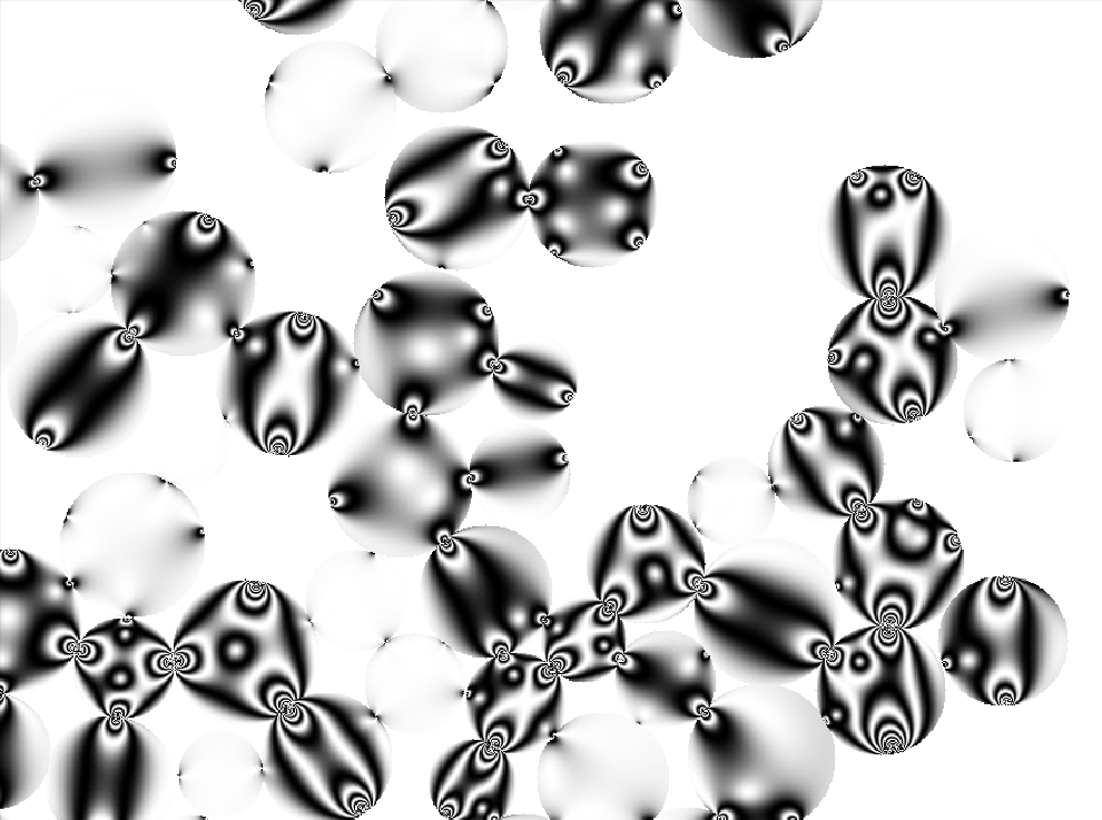
The inverse method analysis provides a quantitative estimation of the force network inside a granular media made in a photoelastic material. With such analysis, the contact force's magnitude and orientation can be determined under some assumptions. The main idea of the inverse method is to generate a numerical photoelastic picture that matches the experimental one like illustrated below (the experimental picture comes from the Matlab implementation of the method).

To achieve a good matching an optimization procedure is used, this procedure required a numerical computation of the photoelastic signal in the granular media. For cylindrical particles, such an analytical expression of this signal can be obtained using the theory of elasticity and the theory of photoelasticity.

The different steps of this method are: 1. Detecting the particles; 2. Getting an initial guess of contact forces; 3. Fitting the numerical and experimental photoelastic pictures.

2. Inverse method procedure

About the first step every detail is given on the dedicated page and nothing has to be added. For the initial guess of the contact force, the $G^2$ value defined in the gradient analysis is used. Depending on the quality of the pictures, some manipulation based on this $G^2$ can be done in order to distribute the force over the contacts. A good initial force guessing increases the optimization procedure in speed and results quality. The forces determination occurs with an optimization procedure. This procedure is described hereafter as it is specific to the inverse method analysis.

2.1 Analytical expressions of the photoelastic signal

All the steps needed to retrieve the stress field inside a cylindrical particle (called disks for the remainder of this document) submitted to multiple loads are available in different sources [1,2]. Here we briefly summarized the assumptions, the principle and give the final results.

The assumptions required to obtain the stress field inside the disk are: 1. Condition of equilibrium (force and torque balance); 2. Linear elasticity; 3. Plane strain; 4. Conditions of compatibility; 5. No body-forces (gravity...);

The stress field inside the disk is obtained by the superposition of: 1. A simple radial stress distribution for each load $i$: $\sigma_{r_i} = -\frac{2f_{i}}{h\pi}\frac{\cos\theta_i}{r_i}$; 2. An uniform tension to ensure a stress-free boundary: $\sigma_{xx} = \sigma_{yy} = \sum_{i=1}^{N}\frac{f_{i}}{\pi h d}\cos\left(\theta_{1,i}+\theta_{2,i}\right)$.

Of course for the summation, the stress tensors have to be expressed in the same coordinates system.

In a circular polariscope, the light intensity is a function of the difference between the two principal stress. This difference is equal to $\sigma_{1}-\sigma_{2} = \sqrt{\left(\left(\sigma_{xx}-\sigma_{yy}\right)^2+\left(2\sigma_{xy}\right)^2\right)}$ which is easely derivate from the Mohr's circle for 2D stress.

2.2 Guessing initial forces value

From the position and dimensions of the disk, it is easy to construct a possible contact network based on geometrical considerations. A contact occurs if the distance between the two disk centers is lower than the sum of the two radii increased by a small tolerance to overcome imprecision from the detection step. This provides the location of all possible contact forces acting on each disk, but it includes some false contacts (due to the tolerance) or non-force-bearing (which does not transmit any load).

A correct result of the optimization procedure required a good initial force distribution. The gradient analysis provides the $G^2$ value which is proportional to the sum of the contact force magnitude $\sum_i|F_i|$ acting on the disk. To provide the initial guess of force distribution, two methods are available depending on the quality of the pictures.

In the case of high-quality pictures (resolution and contrast), a $G^2_i$ at each contact $i$ can be computed using a small region of interest located near the contact point. The false and non-force-bearing contacts are eliminated if their $G^2_i$ value is lower than a threshold value on both contacting disks. The sum of the contact force magnitude is then distributed on the remaining contacts in proportion to the value of $G^2_i$. [1]

In the case of low-quality pictures, each possible combination of active contact is provided to the optimization procedure. The sum of the contact force magnitude is equally distributed over the active contacts. This approach is slower than the previous one and only gives good results when the contact force are almost equally distributed over the active contacts. To overcome the second drawback the fitting procedure will consider all the granular media to propagate the fitted forces on the adjacent disk when the optimization procedure succeeds (PhD Thesis of O. Lantsoght, Université Catholique de Louvain, 2019).

JK: I'm currently trying an idea to use betweenness centrality as an initial guess (based on this ) maybe I can add an outlook here...

2.3 Optimization procedure

The optimization procedure uses the force's magnitude and orientation as parameters and tries to minimize the difference between the computed photoelastic signal and the picture of the disk. Different methods exist to compare two images, among them we have the Mean Squared Error (MSE) or the Structural Similarity Index (SSIM) [3,4]. The main advantage of the MSE is the speed of computation but it considers the image globally. On the opposite, the SSIM is slower but considers the region of the image to take into account its structure. Presently, for this application, both comparison criteria are similar, they are globally good but in some cases failed to detect that the images do not match at all.

Comparison of SSIM and MSE index value on some particles (from Fig.1). The SSIM value range is between 0 and 1. The optimization process is a minimization process so we compute 1-SSIM.

The optimization algorithm must be able to handle non-linear problems and possibly constraints to impose force and torque balance. If the chosen algorithm does not handle constraints, the equilibrium condition can either be imposed by reducing the free parameters by 3 [1] or simply be skipped and assuming that the fitted pictures impose the torque and force balance.

2.4 Force propagation

In the case of low-quality pictures, the initial guess of the forces distribution may be not precise enough to converge toward correct results. A correct result is identified by a threshold value to reach by the MSE or SSIM value.

To improve the initial guess of the forces provided to the optimizer, the forces identified on some disks are applied to the adjacent disk using Newton's third law. Then the optimization procedure is called with all possible combinations of active contact (the propagated contact force is always active). If an optimization procedure succeeds, the newly identified forces are propagated to their neighbors. This procedure is illustrated below.

The forces must be identified in order to reproduce the photoelastic signal of Fig.2. Figure 3 shows the gradient value at each point of the particles, the G2 value on each particle, and the sum of the contact force magnitude.

The optimizer is called for all particles with all combinations of active contact. The sum of the contact force magnitude is evenly distributed on all active contact. Figure 4 give all possible combination for particle number 1 (top left), the photoelastic signal obtained after optimization, and the SSIM value. The Fig.5 shows the result of this first run of optimization, the solved particles are the green ones.

The next iteration of optimization will be done on particles number 5 and 7 as they both have a solved contact from the neighbors (particles 3 and 4). All possible combinations for particle number 5 are illustrated in Fig.6. note that the contact force value with particles 3 and 4 are the same for all combinations. After this step of iteration, the particle 5 is solved but not the 7 (Fig.7).

The next iteration of optimization will only be carried out on particles 6 and 7. The only unknowns are the contact forces with the walls. This step allows us to retrieve the photoelastic response of Fig.3.

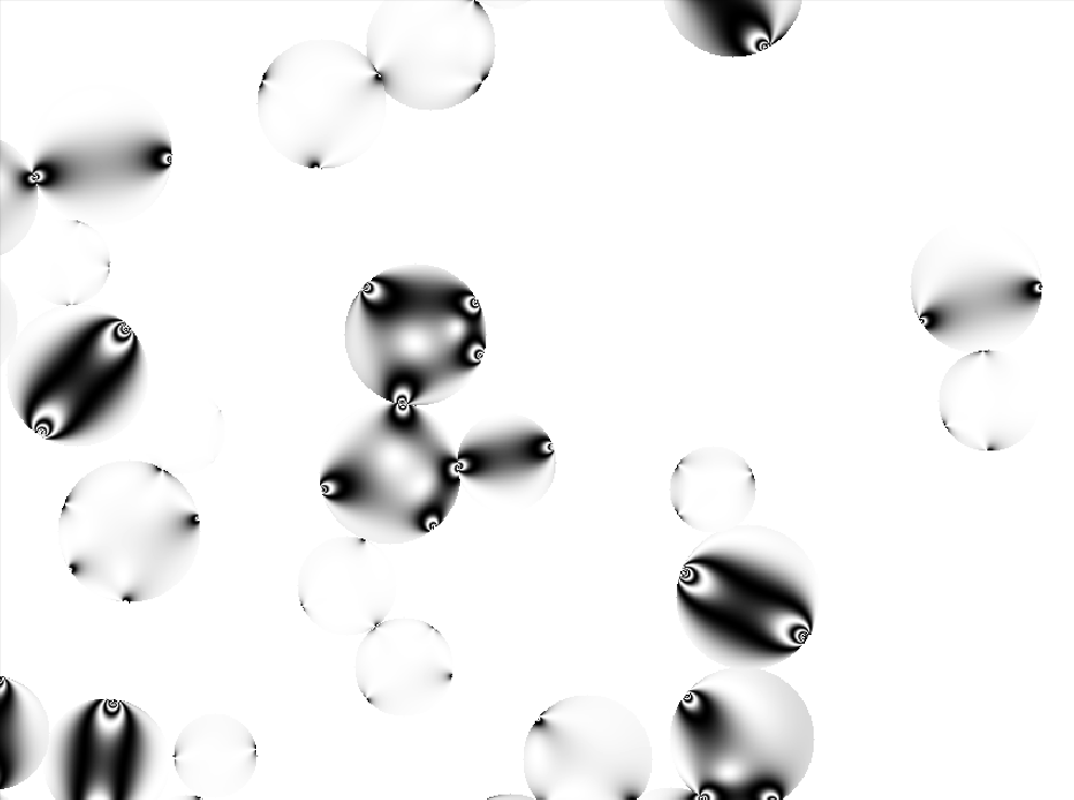
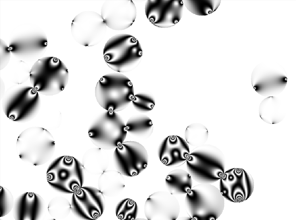
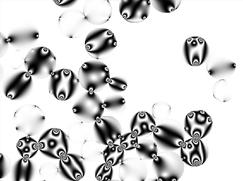
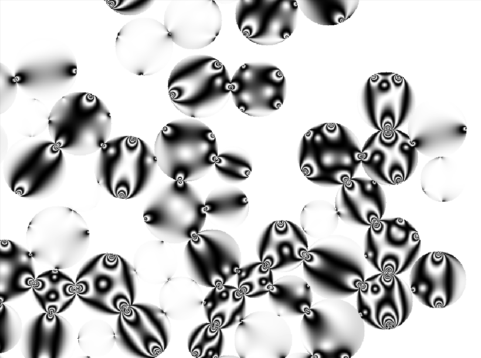
The following pictures show the same algorithm on a more complex example. The first picture is the experimental photoelastic response. The next pictures illustrate the iterations 1 to 5, after that the algorithm does not reach the specified SSIM value on any new particle and the optimization process ends.

3. Examples

Force propagation

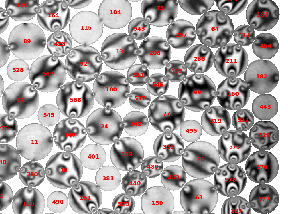
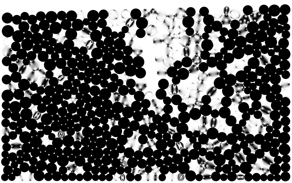
The following pictures show the picture of an experiment (left) and the corresponding photoelastic signal (right). In this experiment, the frame is vertically vibrated while the blender (stadium black shape at the center) oscillates by rotating around its upper extremity (that does not move vertically). In this experiment a circular bright-field polariscope is used, this is why the background is white.

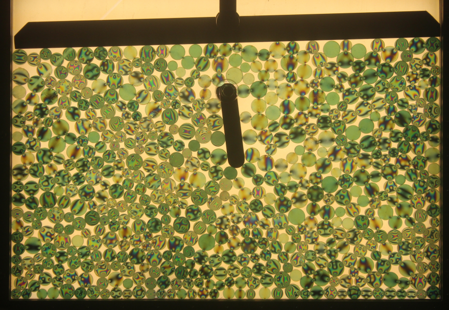
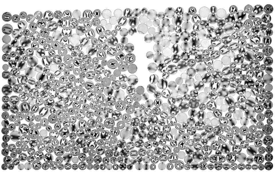
The quality of the picture only allows us to correctly identify good enough initial forces to converge the photoelastic signal on disks with simple force distribution (top left figure). The force propagation procedure allows to reach convergence on more disks with more complex loading.

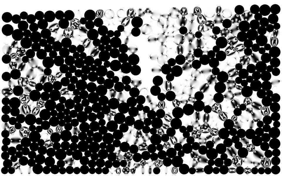
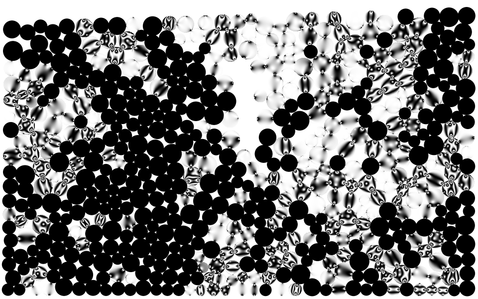
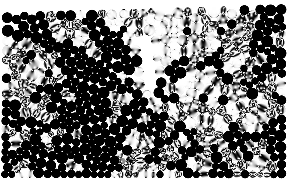
Eventually, the procedure did not succeed to reach convergences on all disks (bottom right figure) for reasons related to picture quality as well as assumption violation: * Some disks show so close fringes that the picture of the signal is just gray, leading to completely wrong forces estimation; * Some disks show large deformations (up to 10% of their radius), in this situation the analytical expression of the stress is no more valid; * The experiment is dynamic, some disks show residual constraints from a previous contact.

To improve the current result, it may be possible to manually provide some initial force for the optimization procedure for some disks. If the optimization succeeds, the force propagation procedure can be restarted from the newly converged disks.

4. Reference

[1] K. E. Daniels, J. E. Kollmer, and J. G. Puckett, "Photoelastic force measurements in granular materials." Review of Scientific Instruments, vol. 88, no. 5, May 2017.

[2] S. Timoshenko and J. N. Goodier, Theory of Elasticity, 3rd ed. New-York: McGraw-Hill, 1970.

[3] Z. Wang, A. C. Bovik, H. R. Sheikh, and E. P. Simoncelli, “Image quality assessment : from error visibility to structural similarity,” IEEE Transactions on Image Processing, vol. 13, pp. 600–612, Apr. 2004.

[4] Z. Wang and A. C. Bovik, "Mean squared error: love it or leave it? - A new look at signal fidelity measures," IEEE Signal Processing Magazine, vol. 26, no. 1, pp. 98-117, Jan. 2009.

4.1 Implementation

Photo-elastic Grain Solver (PEGS): 1. Matlab implementation: Git project [1]. 2. Python implementation: Git project (based on [1]).

<go back to home